Vector Database

You might have heard news recently about vector database startups raising millions just after writing their PPT, or open-source vector databases making headlines on Hackernews for their simple code. In the past few months, AI applications have been developing rapidly, driving the boom in AI technology stacks, and vector databases are one of the hottest.

I recently needed to learn about vector databases while developing two open-source projects: ChatFiles and VectorHub. After understanding the main vector databases and search algorithms, I decided to organize this knowledge into an article to help others.

GPT's Limitations

Over the past few months, we've been in the middle of an AI revolution, with GPT-3.5/4 being the most impressive. While GPT-3.5/4 brings us endless amazement, its natural flaws and many limitations also give developers headaches. For example, the context size limit on the input side troubles many developers and users. The gpt-3.5-turbo model has a limit of 4K tokens (~3000 words), meaning users can input at most 3000 words for GPT to understand and reason answers.

Some might wonder: ChatGPT has conversation memory, so even if it has input token limits, it shouldn't matter. I can just split my text content into multiple inputs, and it will naturally remember my previous conversations, thus removing the token limit.

This idea is not quite right. GPT as an LLM model has no memory function. The so-called memory function is just developers storing conversation records in memory or databases. When you send a message to the GPT model, the program automatically combines recent conversation records (limited to 4096 tokens based on word count) through prompts into the final question and sends it to ChatGPT. Simply put, if your conversation memory exceeds 4096 tokens, it will forget previous conversations. This is currently an insurmountable flaw of GPT in complex tasks.

Currently, different models have different token limits. GPT-4 has a 32K token limit, while the current largest token limit is Claude's 100K, meaning you can input about 75,000 words of context to GPT, enough for GPT to directly understand an entire Harry Potter book and answer related questions.

But does this solve all our problems? The answer is no. First, Claude's example shows that GPT processing 72K tokens of context takes 22 seconds to respond. If we have GB-level or larger documents that need GPT understanding and Q&A, current computing power can hardly provide a good experience. More importantly, current GPT API pricing is based on tokens, so the more context input, the more expensive it becomes.

This situation is similar to early developers facing the dilemma of developing applications when memory was only a few MB or even KB. First, 'memory' is expensive, and second, 'memory' is too small. So before GPT models have revolutionary progress in performance, cost, and attention mechanisms, developers must face the challenge of bypassing GPT token limits.

The Rise of Vector Databases

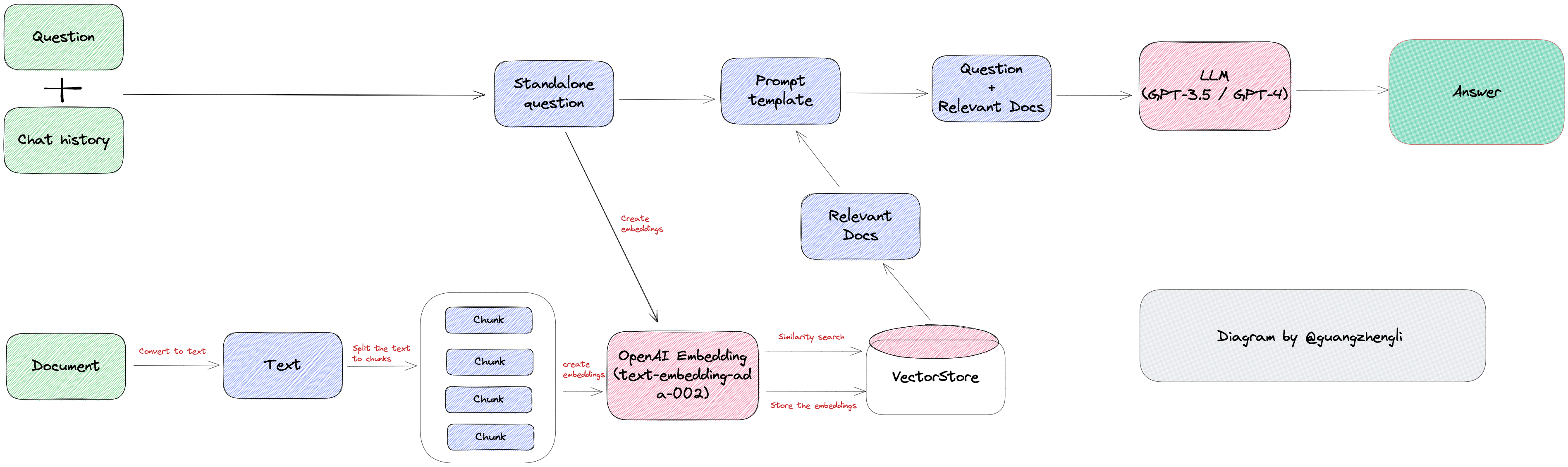
Under GPT model limitations, developers have to find other solutions, and vector databases are one of them. The core idea of vector databases is to convert text into vectors, store vectors in databases, and when users input questions, convert questions into vectors, search for the most similar vectors and context in the database, and finally return text to users.

When we have a document that needs GPT processing, such as customer service training materials or operation manuals, we can first convert all content of this document into vectors (this process is called Vector Embedding). Then when users ask related questions, we convert user search content into vectors, search for the most similar vectors in the database, match the most similar contexts, and finally return the context to GPT. This not only greatly reduces GPT's computation, thus improving response speed, but more importantly reduces costs and bypasses GPT's token limits.

For example, if we have a long conversation with ChatGPT, we can save all conversations as vectors. When we ask ChatGPT questions, we can convert questions into vectors to perform semantic search on all past chat records, find the most relevant 'memories' to the current question, and send them together to ChatGPT, greatly improving GPT's output quality.

Vector databases' role certainly doesn't stop at text semantic search. In traditional AI and machine learning scenarios, they also include face recognition, image search, voice recognition, and other functions. But undeniably, this round of vector database popularity is precisely because they greatly help AI gain understanding and maintain long-term memory to perform complex tasks. For example, you can try LangChainJs's document search/Q&A function to feel its charm, or try my open-source projects VectorHub and ChatFiles, where you can upload documents or base on web documents and ask document-related questions. These functions are all products based on Vector Embedding and vector databases.

Vector Embeddings

For traditional databases, search functions are all based on different indexing methods (B Tree, inverted index, etc.) plus exact matching and sorting algorithms (BM25, TF-IDF, etc.). The essence is still based on exact text matching. This indexing and search algorithm is very suitable for keyword search functions, but very weak for semantic search functions.

For example, if you search for "puppy," you can only get results with "puppy" keywords, and cannot get results like "Corgi" or "Golden Retriever" because "puppy" and "Golden Retriever" are different words. Traditional databases cannot identify their semantic relationship, so traditional applications need to manually tag relationships between "puppy" and "Golden Retriever" to achieve semantic search. The process of generating and selecting features is also called Feature Engineering, which is the process of transforming raw data into features that better express the essence of the problem.

But if you need to process unstructured data, you'll find that the number of unstructured data features starts to expand rapidly. For example, if we process images, audio, video data, this process becomes very difficult. For example, for images, you can tag features like color, shape, texture, edges, objects, scenes, etc., but there are too many features, and it's difficult to tag them manually. So we need an automated way to extract these features, which can be achieved through Vector Embedding.

Vector Embedding is generated by AI models (such as large language models LLM). It generates high-dimensional vector data based on different algorithms, representing different features of data. These features represent different dimensions of data. For example, for text, these features might include vocabulary, grammar, semantics, emotion, mood, topics, context, etc. For audio, these features might include pitch, rhythm, tone, timbre, volume, speech, music, etc.

For example, for text vectors, they can be generated through OpenAI's text-embedding-ada-002 model. Image vectors can be generated through the clip-vit-base-patch32 model, and audio vectors can be generated through the wav2vec2-base-960h model. These vectors are all generated by AI models, so they all have semantic information.

For example, if we use the text-embedding-ada-002 model to perform text embedding on the sentence "Your text string goes here," it will generate a 1536-dimensional vector. The result looks like: "-0.006929283495992422, -0.005336422007530928, ... -4547132266452536e-05,-0.024047505110502243", which is an array of length 1536. This vector contains all features of this sentence, including vocabulary and grammar. We can store it in a vector database for later semantic search.

Features and Vectors

Although the core of vector databases lies in similarity search, before understanding similarity search in depth, we need to understand the concepts and principles of features and vectors in detail.

Let's think about a question first: Why can we distinguish different items and things in life?

From a theoretical perspective, this is because we identify types by recognizing different features between different things. For example, to distinguish different types of puppies, we can distinguish them by features like body size, hair length, nose length, etc. In the photo below, arranged by body size, you can see that larger dogs are closer to the right side of the coordinate axis, thus getting a one-dimensional coordinate and corresponding values for the body size feature, getting each dog's position in the coordinate system from numbers 0 to 1.

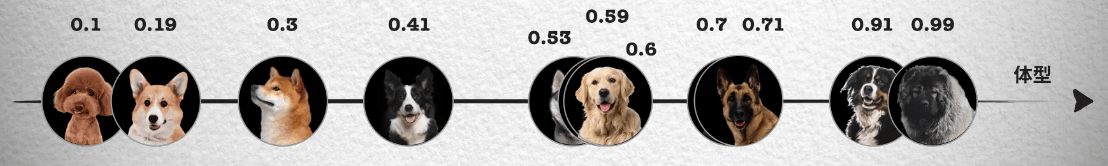
However, relying solely on body size feature is not enough. Like in the photo, Husky, Golden Retriever, and Labrador have very similar body sizes, and we cannot distinguish them. So we continue to observe other features, such as hair length.

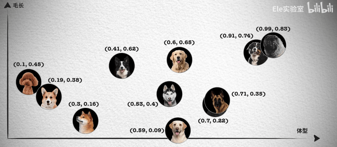
This way, each dog corresponds to a two-dimensional coordinate point, and we can easily distinguish Husky, Golden Retriever, and Labrador. If we still cannot distinguish German Shepherd and Rottweiler well, we can continue to distinguish from other features, such as nose length, thus getting a three-dimensional coordinate system and each dog's position in the three-dimensional coordinate system.

In this case, as long as there are enough features, we can distinguish all dogs and finally get a high-dimensional coordinate system. Although we cannot imagine what a high-dimensional coordinate system looks like, in arrays, we just need to keep adding numbers to the array.

Actually, as long as there are enough dimensions, we can distinguish all things. Everything in the world can be represented by a multi-dimensional coordinate system, and they all correspond to a coordinate point in a high-dimensional feature space.

So what does this have to do with similarity search? You'll find that in the two-dimensional coordinate above, German Shepherd and Rottweiler's coordinates are very close, which means their features are also very close. We know that vectors are mathematical structures with magnitude and direction, so we can represent these features with vectors. This way, we can judge their similarity by calculating the distance between vectors. This is similarity search.

The above images and detailed explanations come from this video. This video series also includes some similarity search algorithms introduced below. If you're interested in vector databases, I highly recommend watching this video.

Similarity Search

Since we know we can judge similarity by comparing distances between vectors, how do we apply this to real scenarios? If we want to find the most similar vector to a certain vector in massive data, we need to compare and calculate each vector in the database, but this computation is huge. So we need efficient algorithms to solve this problem.

There are many efficient search algorithms, and their main idea is to improve search efficiency through two methods:

Reduce vector size — through dimensionality reduction or reducing the length of vector value representation.
Narrow search scope — can be achieved by clustering or organizing vectors into tree-based, graph-based structures, and limiting search scope to only the closest clusters, or filtering through the most similar branches.

Let's first introduce the core concept shared by most algorithms: clustering.

K-Means and Faiss

After saving vector data, we can first cluster the vector data. For example, in the figure below in a two-dimensional coordinate system, 4 clustering centers are defined, then each vector is assigned to the nearest clustering center. Through clustering algorithms continuously adjusting clustering center positions, vector data can be divided into 4 clusters. During each search, we only need to first determine which cluster the search vector belongs to, then search within that cluster, thus reducing the search range from 4 clusters to 1 cluster, greatly reducing the search scope.

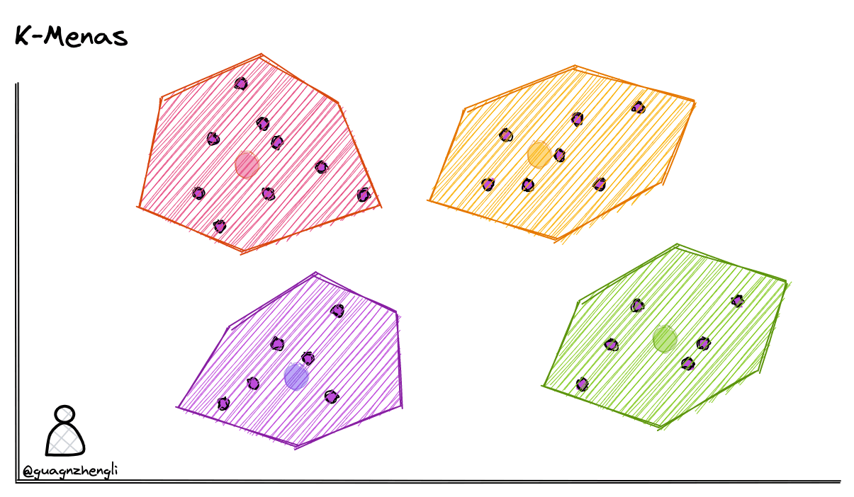
Common clustering algorithms include K-Means, which can divide data into k categories, where k is pre-specified. Here are the basic steps of the k-means algorithm:

Choose k initial clustering centers.
Assign each data point to the nearest clustering center.
Calculate the new center for each cluster.
Repeat steps 2 and 3 until clustering centers no longer change or reach maximum iterations.

But this search method also has some drawbacks. For example, during search, if the search content happens to be in the middle of two classification regions, it's very likely to miss the most similar vector.

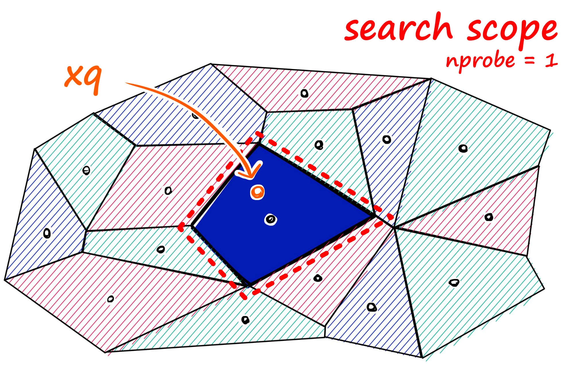
In real situations, vector distribution won't be as clearly distinguished as in the figure. Often, region boundaries are adjacent, like in the Faiss algorithm figure below.

We can imagine vectors contained in Voronoi cells - when a new query vector is introduced, first measure its distance to centroids, then limit the search scope to the cell where that centroid is located.

To solve the possible omission problem during search, we can dynamically adjust the search scope. For example, when nprobe = 1, only search the nearest clustering center; when nprobe = 2, search the nearest two clustering centers. Adjust the nprobe value according to actual business needs.

Actually, except for brute force search which can perfectly find the nearest neighbor, all search algorithms can only make trade-offs between speed, quality, and memory. These algorithms are also called Approximate Nearest Neighbor.

Product Quantization (PQ)

In large-scale datasets, the biggest problem with clustering algorithms is excessive memory usage. This is mainly reflected in two aspects: first, because each vector's coordinates need to be saved, and each coordinate is a floating-point number, the memory usage is already very large. Additionally, clustering centers and each vector's clustering center index need to be maintained, which also consumes a lot of memory.

For the first problem, it can be solved through quantization, which is common lossy compression. For example, in memory, each vector in clustering centers can be represented by the clustering center vector, and maintain a codebook from all vectors to clustering centers, thus greatly reducing memory usage.

But this still cannot solve all problems. In the previous example, clustering centers were divided in a two-dimensional coordinate system. Similarly, in high-dimensional coordinate systems, multiple clustering center points can be defined, continuously adjusted and iterated until multiple stable and convergent center points are found.

But in high-dimensional coordinate systems, we also encounter the curse of dimensionality. Specifically, as dimensions increase, distances between data points grow exponentially. This means that in high-dimensional coordinate systems, more clustering center points are needed to divide data points into smaller clusters to improve classification quality. Otherwise, vectors will be far from their clustering centers, greatly reducing search speed and quality.

But if we want to maintain classification and search quality, we need to maintain a huge number of clustering centers. This brings another problem: the number of clustering center points will grow exponentially with increasing dimensions, causing the number of codebooks we store to increase rapidly, greatly increasing memory consumption. For example, a 128-dimensional vector needs to maintain 2^64 clustering centers to maintain good quantization results, but this codebook storage size already exceeds the memory size for maintaining original vectors.

The solution to this problem is to decompose vectors into multiple sub-vectors, then independently quantize each sub-vector. For example, divide a 128-dimensional vector into 8 16-dimensional vectors, then cluster separately on 8 16-dimensional sub-vectors. Because 16-dimensional sub-vectors only need about 256 clustering centers to get good quantization results, we can reduce the codebook size from 2^64 to 8 * 256 = 2048 clustering centers, thus reducing memory overhead.

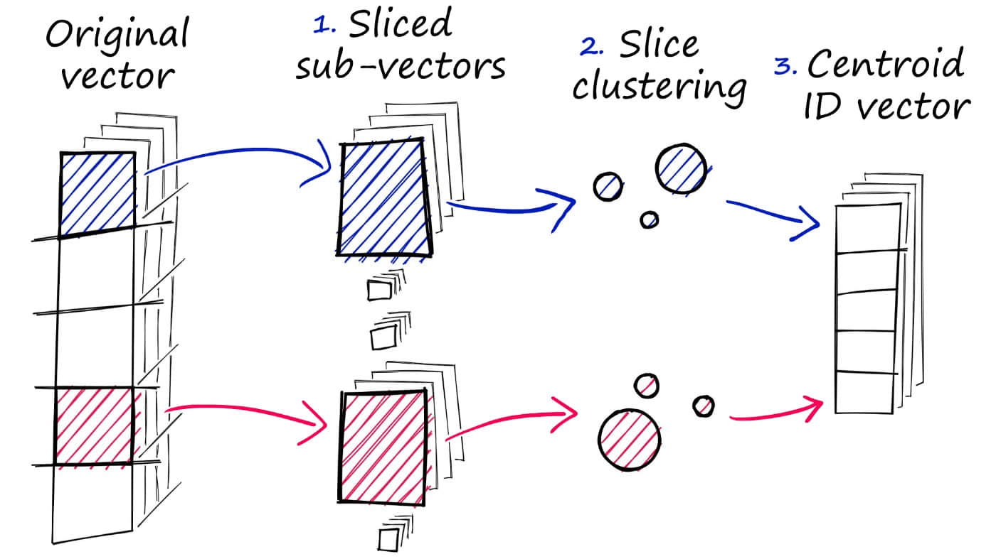
After encoding vectors, we get 8 encoding values. Connecting them gives the final encoding value for that vector. When using, we just need to take these 8 encoding values, then search for corresponding 16-dimensional vectors in 8 sub-codebooks, and combine them using Cartesian product to form a 128-dimensional vector, thus getting the final search result. This is the principle of Product Quantization.

Using the PQ algorithm can significantly reduce memory overhead while speeding up search, but search quality will decrease. But as we said earlier, all algorithms make trade-offs between memory, speed, and quality.

Hierarchical Navigable Small Worlds (HNSW)

Besides clustering, approximate nearest neighbor search can also be implemented by building trees or graphs. The basic idea of this method is that each time a vector is added to the database, first find the most adjacent vector to it, then connect them, thus forming a graph. When searching, start from a node in the graph and continuously perform nearest neighbor search and shortest path calculation until finding the most similar vector.

This algorithm can ensure search quality, but if all nodes in the graph are connected by shortest paths, like the bottom layer in the figure, then during search, all nodes still need to be traversed.

The solution to this problem is similar to the common skip list algorithm. As shown in the figure below, to search the skip list, start from the highest layer and move right along edges with the longest "jumps." If we find the current node's value is greater than the search value, we know we've exceeded the target, so we go to the previous node in the next level.

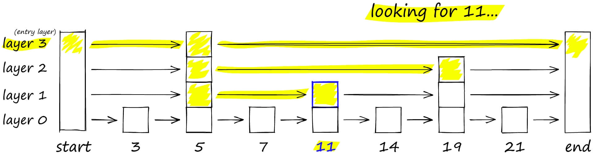
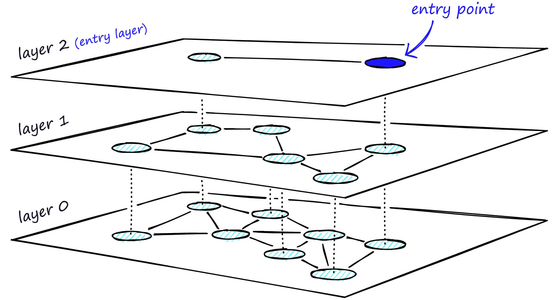
HNSW inherits the same layered format, with the highest layer having longer edges (for fast search) and lower layers having shorter edges (for accurate search).

Specifically, the graph can be divided into multiple layers, each layer being a small world where graph nodes are interconnected. Each layer's nodes connect to the upper layer's nodes. When searching, start from the first layer. Because the first layer has long distances between nodes, search time can be reduced. Then search layer by layer downward. Because the bottom layer has similar nodes interconnected, search quality can be guaranteed, and the most similar vector can be found.

If you're interested in skip lists and HNSW, you can watch this video.

The HNSW algorithm is a classic space-for-time algorithm with high search quality and speed, but it also has large memory overhead because not only do all vectors need to be stored in memory, but a graph structure also needs to be maintained and stored. So this type of algorithm needs to be chosen based on actual scenarios.

Locality Sensitive Hashing (LSH)

Locality Sensitive Hashing is also an indexing technique using approximate nearest neighbor search. Its characteristic is speed while still providing approximate, non-exhaustive results. LSH uses a set of hash functions to map similar vectors to "buckets," making similar vectors have the same hash value. This way, similarity between vectors can be judged by comparing hash values.

Usually, hash algorithms we design aim to reduce hash collisions because hash functions have O(1) search time complexity. But if hash collisions exist, meaning two different keys are mapped to the same bucket, then data structures like linked lists need to be used to resolve conflicts. In this case, search time complexity is usually O(n), where n is the linked list length. So to improve hash function search efficiency, hash collision probability is usually minimized.

But in vector search, our goal is to find similar vectors, so we can specifically design a hash function to make hash collision probability as high as possible, and vectors that are closer or more similar are more likely to collide, so similar vectors will be mapped to the same bucket.

When searching for specific vectors, to find the nearest neighbors of a given query vector, the same hash function is used to "bucket" similar vectors into hash tables. The query vector is hashed to a specific table, then compared with other vectors in that table to find the closest match. This approach is much faster than searching the entire dataset because there are far fewer vectors in each hash table bucket than in the entire space.

So how should this hash function be designed? For better understanding, let's explain from a two-dimensional coordinate system first. As shown in the figure below, in a two-dimensional coordinate system, we can randomly generate a line to divide the two-dimensional coordinate system into two regions, thus judging whether vectors are similar by determining if they're on the same side of the line. For example, in the figure below, by randomly generating 4 lines, we can use 4 binary numbers to represent a vector's position, such as A and B representing vectors in the same region.

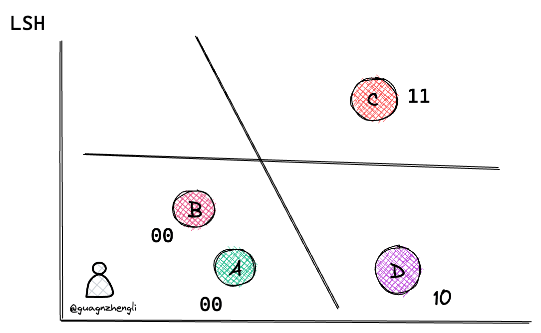
The principle is simple: if two vectors are close, the probability of them being on the same side of the line will be high. For example, the probability of a line passing through AC is much greater than the probability of a line passing through AB. So the probability of AB being on the same side is much greater than the probability of AC being on the same side.

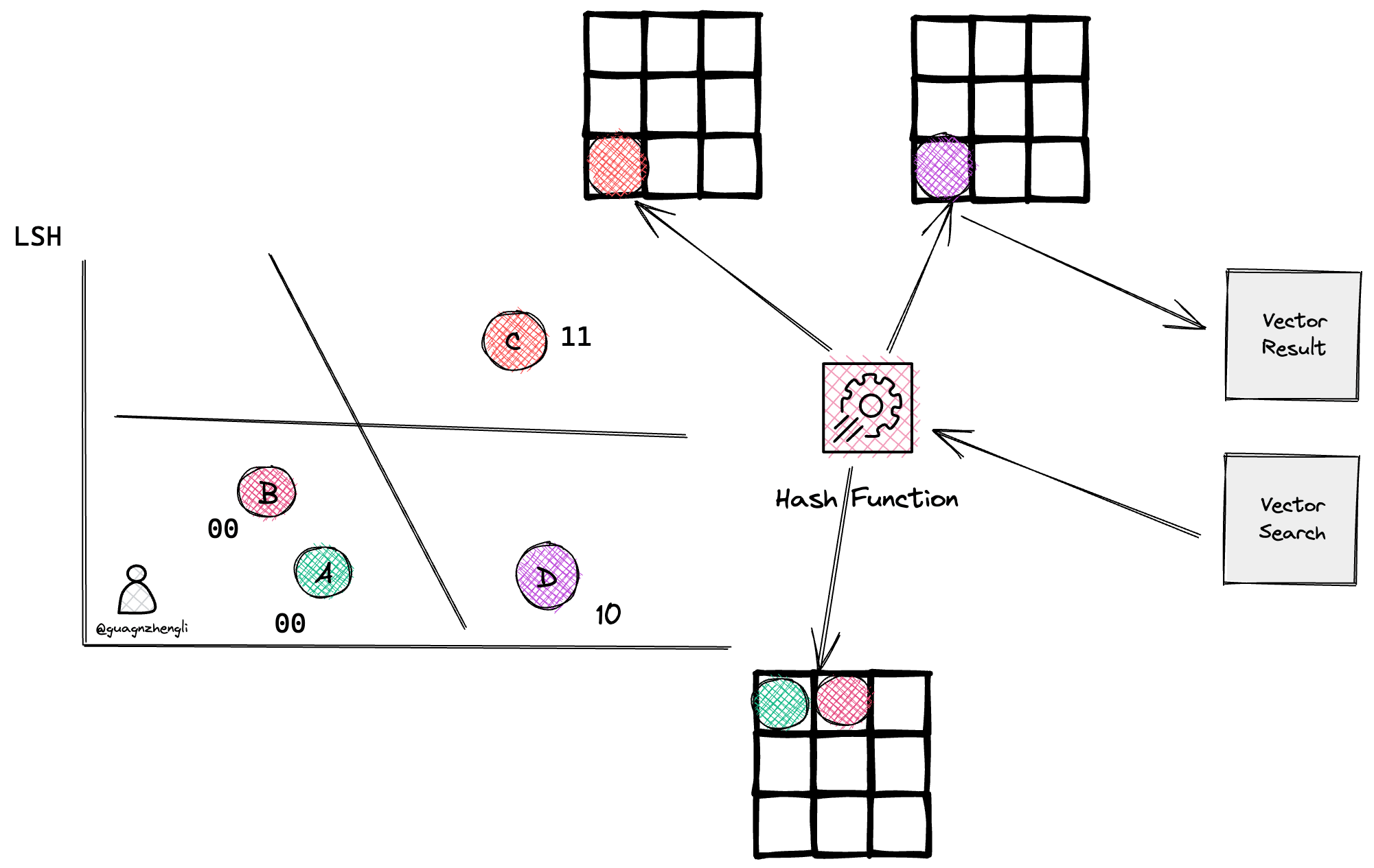
When searching for a vector, hash function calculation is performed again on this vector to get the same bucket's vectors, then brute force search is used to find the closest vector. As shown in the figure below, if a vector is searched and gets a value of 10 through the hash function, it will directly find similar vector D in the same bucket, greatly reducing search time.

For more details about the LSH algorithm, you can refer to this blog.

Random Projection for LSH

If similarity can be distinguished by randomly generated lines in a two-dimensional coordinate system, then similarly, in a three-dimensional coordinate system, we can randomly generate a plane to divide the three-dimensional coordinate system into two regions. In multi-dimensional coordinate systems, we can also randomly generate a hyperplane to divide the multi-dimensional coordinate system into two regions, thus distinguishing similarity.

But in high-dimensional space, distances between data points are often very sparse, and distances between data points grow exponentially with increasing dimensions. This results in many calculated buckets, with the most extreme case being one vector per bucket, and very slow calculation speed. So in actual LSH algorithm implementation, random projection is considered to project high-dimensional space data points to low-dimensional space, thus reducing calculation time and improving query quality.

The basic idea behind random projection is to use a random projection matrix to project high-dimensional vectors into low-dimensional space. A matrix composed of random numbers is created, with size being the desired target low-dimensional value. Then, the dot product between input vectors and the matrix is calculated, resulting in a projected matrix that has fewer dimensions than original vectors but still retains similarity between them.

When we query, the same projection matrix is used to project query vectors to low-dimensional space. Then, projected query vectors are compared with projected vectors in the database to find nearest neighbors. Since data dimensionality is reduced, the search process is much faster than searching in the entire high-dimensional space.

The basic steps are:

Randomly select a hyperplane from high-dimensional space and project data points onto that hyperplane.
Repeat step 1, select multiple hyperplanes, and project data points onto multiple hyperplanes.
Combine projection results from multiple hyperplanes into a vector as representation in low-dimensional space.
Use hash functions to map vectors in low-dimensional space to hash buckets.

Similarly, random projection is also an approximate method, and projection quality depends on the projection matrix. Usually, the more random the projection matrix, the better its mapping quality. But generating truly random projection matrices can be computationally expensive, especially for large datasets. For more details about RP for LSH algorithm, you can refer to this blog.

Similarity Measurement

We've discussed different search algorithms for vector databases above, but haven't discussed how to measure similarity. In similarity search, we need to calculate distances between two vectors, then judge their similarity based on distance.

So how do we calculate vector distances in high-dimensional space? There are three common vector similarity algorithms: Euclidean distance, cosine similarity, and dot product similarity.

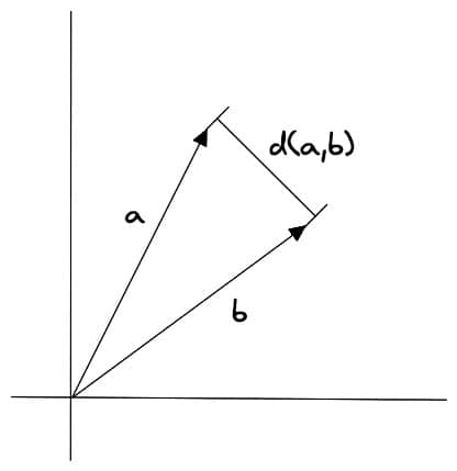
Euclidean Distance

Euclidean distance refers to the distance between two vectors, with the calculation formula:

$d(\mathbf{A}, \mathbf{B}) = \sqrt{\sum_{i=1}^{n}(A_i - B_i)^2}$

Where $\mathbf{A}$ and $\mathbf{B}$ represent two vectors, and $n$ represents vector dimension.

The advantage of Euclidean distance algorithm is that it can reflect absolute distance between vectors, suitable for similarity calculations that need to consider vector length. For example, in recommendation systems, we need to recommend similar products based on users' historical behavior, which requires considering the quantity of users' historical behavior, not just similarity of users' historical behavior.

Cosine Similarity

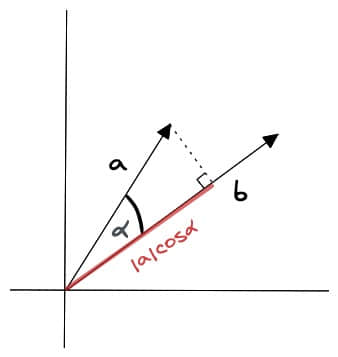
Cosine similarity refers to the cosine value of the angle between two vectors, with the calculation formula:

$\cos(\theta) = \frac{\mathbf{A} \cdot \mathbf{B}}{|\mathbf{A}| |\mathbf{B}|}$

Where $\mathbf{A}$ and $\mathbf{B}$ represent two vectors, $\cdot$ represents vector dot product, and $|\mathbf{A}|$ and $|\mathbf{B}|$ represent the magnitudes of the two vectors.

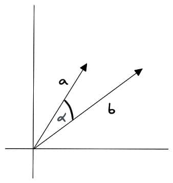
Cosine similarity is not sensitive to vector length and only focuses on vector direction, making it suitable for high-dimensional vector similarity calculations. For example, semantic search and document classification.

Dot Product Similarity

Vector dot product similarity refers to the dot product value between two vectors, with the calculation formula:

$\mathbf{A} \cdot \mathbf{B} = \sum_{i=1}^{n}A_i B_i$

Where $\mathbf{A}$ and $\mathbf{B}$ represent two vectors, and $n$ represents vector dimension.

The advantage of dot product similarity algorithm is that it's simple and easy to understand, fast to calculate, and considers both vector length and direction. It's suitable for many practical scenarios, such as image recognition, semantic search, and document classification. But dot product similarity algorithm is sensitive to vector length, so it may have problems when calculating high-dimensional vector similarity.

Each similarity measurement algorithm has its advantages and disadvantages, and developers need to choose based on their data characteristics and business scenarios.

Filtering

In actual business scenarios, we often don't need to perform similarity search in the entire vector database, but filter through some business fields before querying. So vectors stored in databases often need to include metadata, such as user ID, document ID, and other information. This way, during search, we can filter search results based on metadata to get final results.

For this, vector databases usually maintain two indexes: one is the vector index, and the other is the metadata index. Then, metadata filtering is performed before or after the similarity search itself, but in either case, there are difficulties that can slow down the query process.

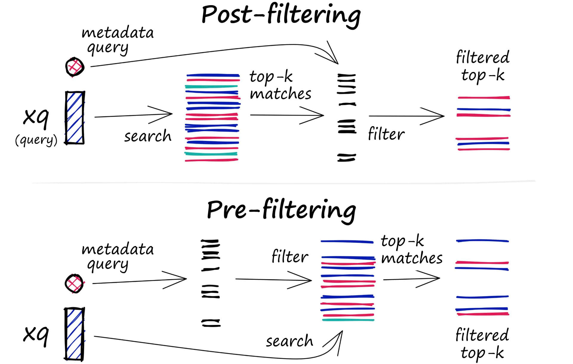
The filtering process can be performed before or after the vector search itself, but each method has its own challenges that may affect query performance:

Pre-filtering: Perform metadata filtering before vector search. While this can help reduce search space, it may also cause the system to ignore relevant results that don't match metadata filtering criteria.
Post-filtering: Perform metadata filtering after vector search is completed. This can ensure all relevant results are considered, filtering out irrelevant results after search completion.

To optimize the filtering process, vector databases use various techniques, such as leveraging advanced indexing methods to handle metadata or using parallel processing to speed up filtering tasks. Balancing the trade-off between search performance and filtering accuracy is crucial for providing efficient and relevant vector database query results.

Vector Database Selection

In this article, I've spent a lot of ink introducing the principles and implementation of similarity search algorithms for vector databases. While similarity search algorithms are indeed the core and key point of vector databases, in actual business scenarios, other factors often need to be considered, such as vector database availability, scalability, security, whether code is open source, whether the community is active, etc.

Distributed

A mature vector database often needs to support distributed deployment to meet large-scale data storage and query requirements. The more data you have, the more nodes you need, and the more errors and failures occur. So distributed vector databases need to have high availability and fault tolerance.

Database high availability and fault tolerance often require implementing sharding and replication capabilities. In traditional databases, sharding is often done through data primary keys or according to business needs. But in distributed vector databases, we need to consider partitioning based on vector similarity to ensure result quality and speed during queries.

Other factors like replica node data consistency, data security, etc., are all factors that distributed vector databases need to consider.

Access Control and Backup

Additionally, whether access control design is sufficient, such as whether new users and permission controls can be quickly added when organizations and businesses develop rapidly, whether new nodes can be quickly added, whether audit logs are complete, etc., are all factors that need to be considered.

Moreover, database monitoring and backup are also important factors. When data failures occur, being able to quickly locate problems and recover data is a factor that mature vector databases must consider.

API & SDK

Compared to the above factor choices, API & SDK might be often overlooked factors, but in actual business scenarios, API & SDK are often the factors developers care about most. Because API & SDK design directly affects developer efficiency and user experience. Excellent API & SDK design can often adapt to different requirement changes. Vector databases are a new field, and when most people aren't clear about requirements in this area, this point is easily overlooked.

Selection

As of now, here are the current vector database choices:

Vector Database	URL	GitHub Star	Language	Cloud
chroma	https://github.com/chroma-core/chroma	7.4K	Python	❌
milvus	https://github.com/milvus-io/milvus	21.5K	Go/Python/C++	✅
pinecone	https://www.pinecone.io/	❌	❌	✅
qdrant	https://github.com/qdrant/qdrant	11.8K	Rust	✅
typesense	https://github.com/typesense/typesense	12.9K	C++	❌
weaviate	https://github.com/weaviate/weaviate	6.9K	Go	✅

Traditional Database Extensions

Besides choosing professional vector databases, extending traditional databases is also a method. Similar to Redis, besides traditional Key Value database uses, Redis also provides Redis Modules, which is a way to extend Redis with new features, commands, and data types. For example, using the RediSearch module to extend vector search functionality.

Similarly, there are PostgreSQL extensions. PostgreSQL provides a way to extend database functionality using extensions, such as pgvector to enable vector search functionality. It not only supports exact and similarity search but also supports similarity measurement algorithms like cosine similarity. Most importantly, it's attached to PostgreSQL, so it can utilize all PostgreSQL features, such as ACID transactions, concurrency control, backup and recovery, etc. It also has all PostgreSQL client libraries, so you can use PostgreSQL clients in any language to access it. This can reduce developers' learning costs and service maintenance costs.

My open-source projects ChatFiles and VectorHub currently use pgvector to implement vector search for GPT document Q&A, based on Supabase's PostgreSQL + pgvector service.

Summary

This article mainly introduces the principles and implementation of vector databases, including basic concepts of vector databases, similarity search algorithms, similarity measurement algorithms, filtering algorithms, and vector database selection. Vector databases are a new field. Currently, most vector database companies' valuations are rapidly growing riding the wave of AI and GPT, but in actual business scenarios, vector database application scenarios are still relatively few. Removing the impetuous exterior, vector database application scenarios still need to be explored by developers and business experts.